A Victron ESS next to an Enphase system is two energy systems sharing one house. Each comes with its own app, and each app is confident about its own half of the truth. To see what is actually going on – where the PV goes, when the batteries cycle, when the grid is touched and at what price – I built a set of Grafana dashboards on my self-hosted stack. This post walks through the panels that turned out to be genuinely useful for monitoring such a hybrid system, and a few traps I fell into on the way.

The dashboard labels are in Luxembourgish; I translate the important ones as we go.

The setup

• Victron side: 3× MultiPlus-II 48/6500 (three-phase ESS), Ekrano GX, two DIY 16 kWh LiFePO4 packs (EEL V6 Pro with JK BMS, 32 kWh in total), three Victron VM-3P75CT energy meters in the roles grid, loads and PV.
• Enphase side: 37 IQ8 microinverters on two roofs, AC-coupled on the Victron AC-out, plus two IQ Battery 5P.
• Data path: Telegraf reads the Ekrano over MQTT into InfluxDB 2 (raw data with limited retention, plus a 1-minute bucket kept indefinitely). openHAB polls the Envoy (per-panel data, Enphase battery) and stores it in its own bucket, together with the day-ahead spot price and the PV forecast. The JK BMS packs are read over an isolated RS485-to-Ethernet converter and published via MQTT, down to individual cell voltages.
• Frontend: Grafana 13, everything self-hosted, no vendor cloud in the loop (Enphase cloud data is pulled nightly as a backup only).

A word of honesty about the data. Two current clamps are not yet where they will end up: the server circuit currently bypasses the loads meter on one phase, and the Enphase IQ batteries sit outside the PV meter, so Venus counts their charging as household load. Everything that depends on the loads meter – household consumption, autarky – is therefore biased for now, and I left those panels out of this post. What you see below is based on the PV, grid and battery measurements, which are correct.

1. Planning: forecast, spot price, state of charge

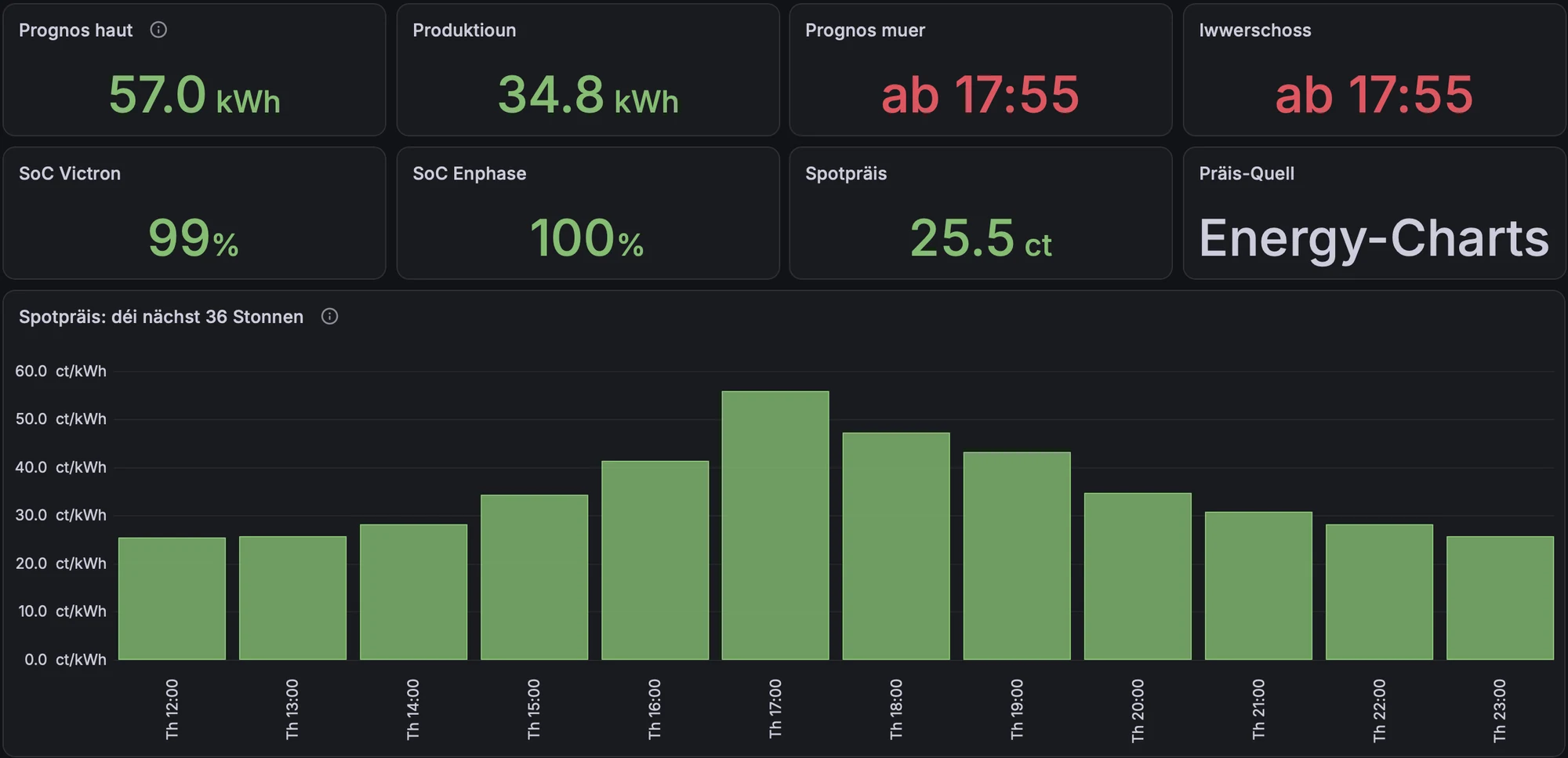
The first dashboard is the one I open in the morning. It shows today’s PV forecast against what has been produced so far, the forecast for tomorrow (here: available from 17:55), both batteries’ state of charge, the current spot price and which price source is active. The price feed queries Energy-Charts and falls back to a second source if that fails; the active source is shown so a silent failover does not go unnoticed.

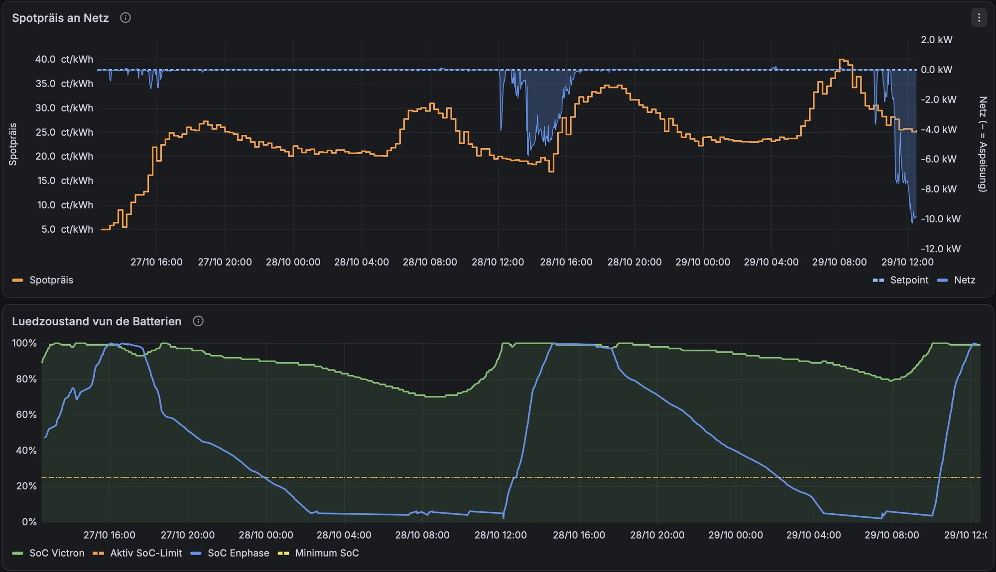
Below it, the spot price is plotted against the grid power. The blue areas are export. On the left you see the classic midday surplus at low prices; on the right, the batteries being sold into the evening price peak. The lower chart shows both batteries’ state of charge – note how differently the small Enphase batteries (blue) and the 32 kWh Victron bank (green) cycle.

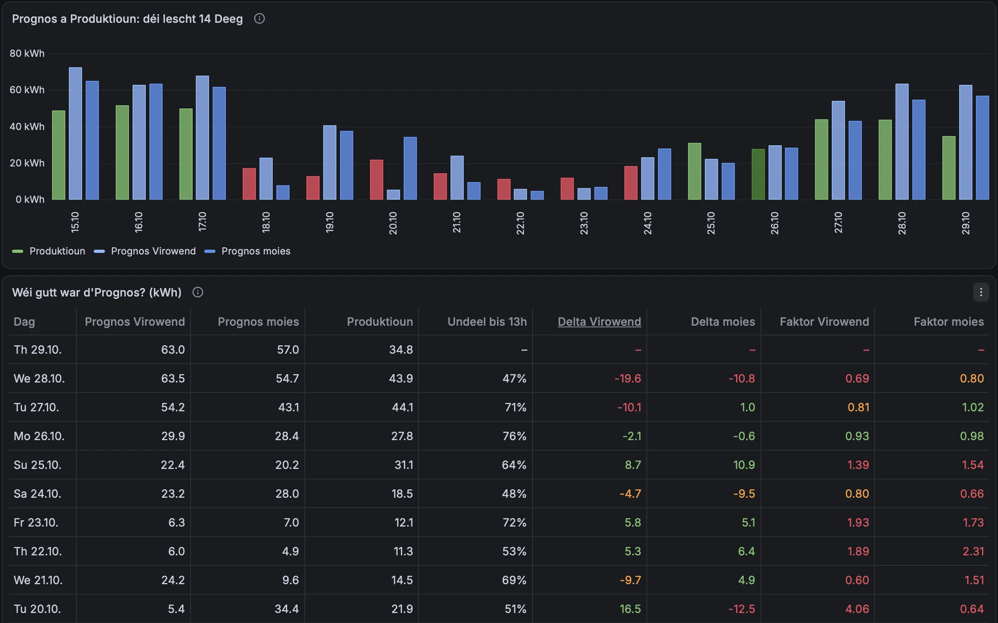
Since the forecast drives decisions (how much to sell in the evening, how much reserve to keep for a dark day), I track how good it is. The table compares the forecast made the evening before and the one made in the morning with actual production. On sunny days the forecast is decent; on overcast days it is off by a factor of two or more in either direction, which is exactly why the battery strategy must not trust a single forecast.

2. PV: per panel and against the sun

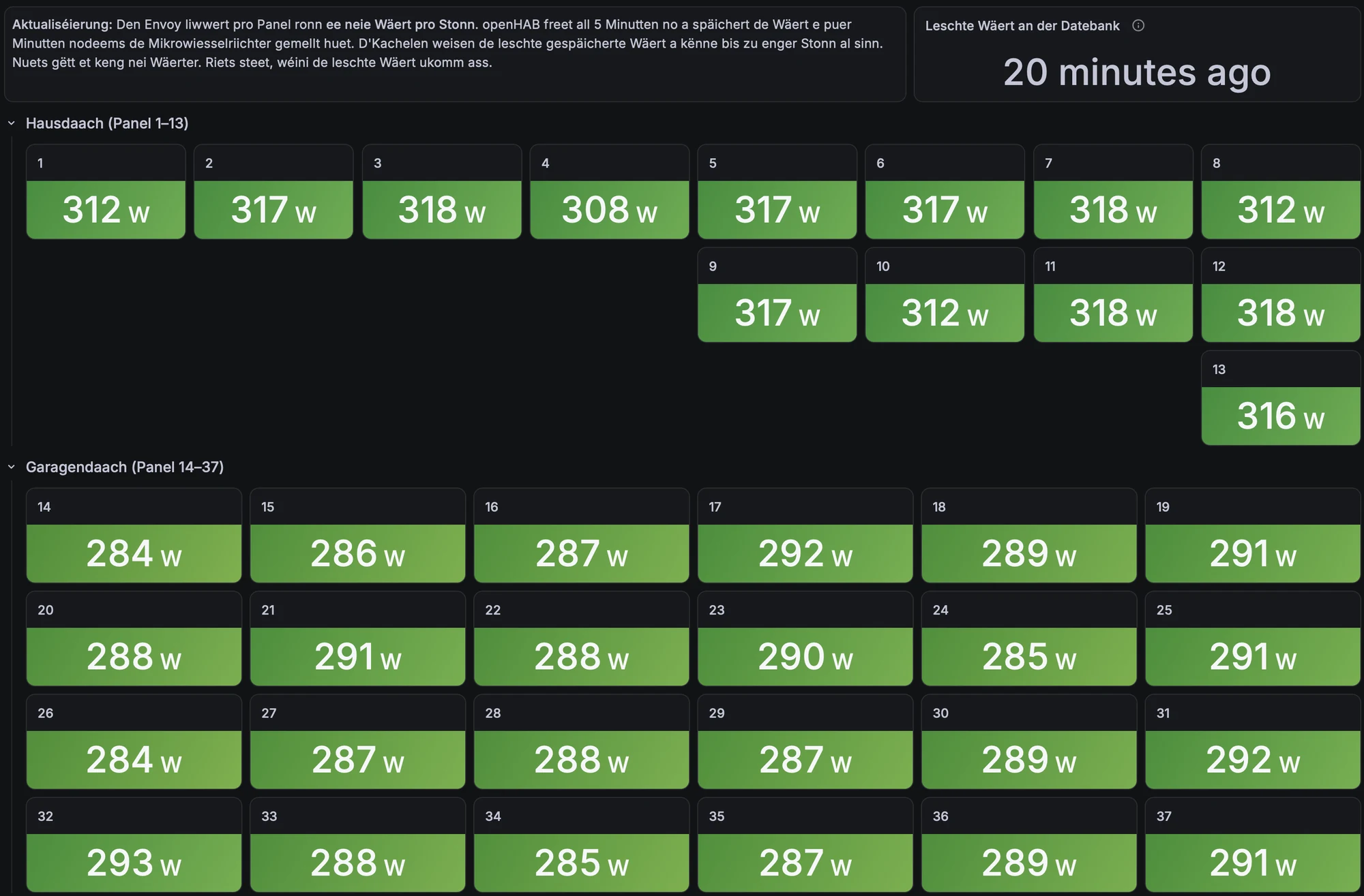
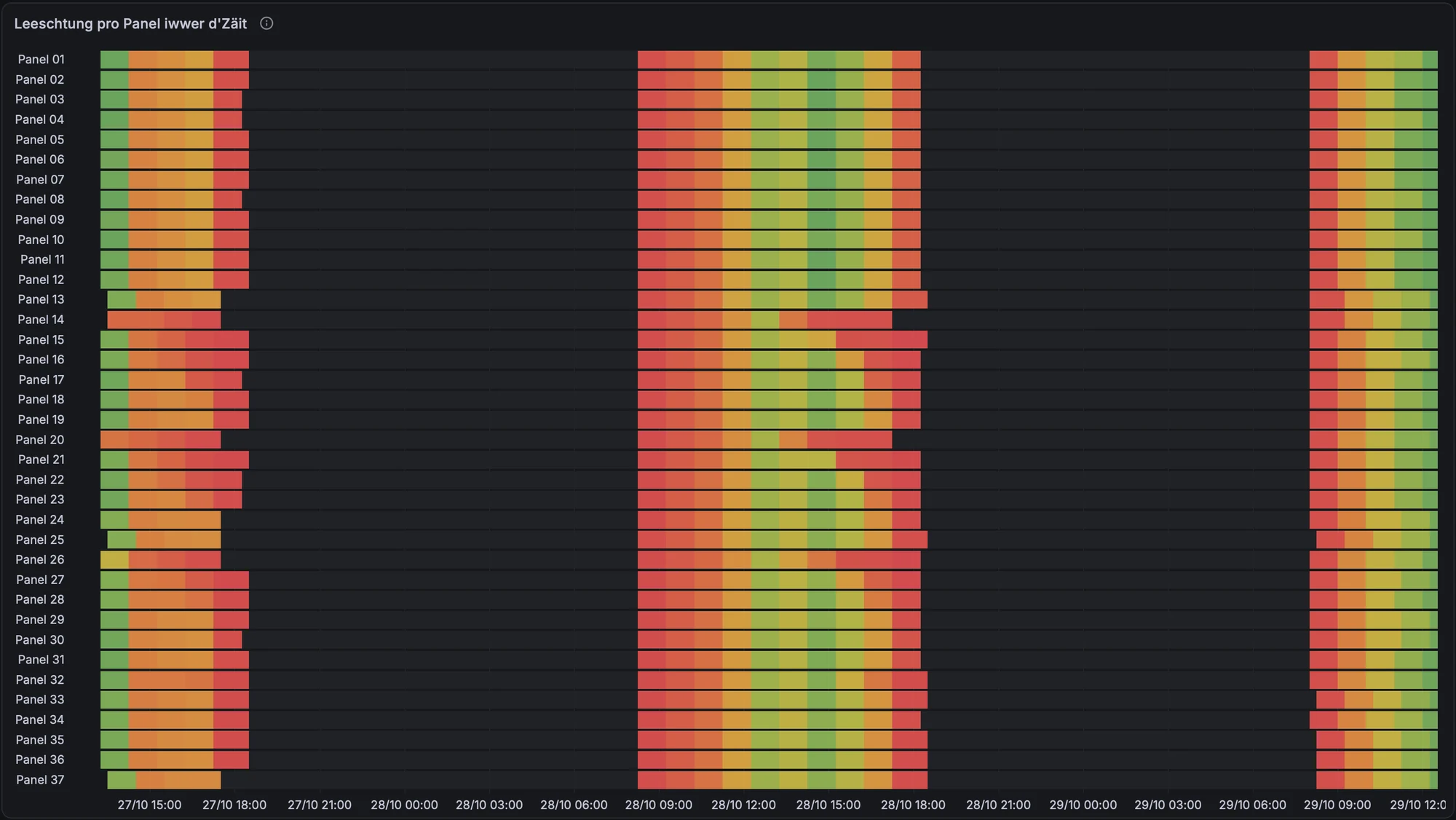
Enphase microinverters report per panel, which makes shading and faults visible that a string inverter would hide. The tiles show the last value per panel, grouped by roof (house roof panels 1–13, garage roof 14–37). The Envoy only updates per-panel data about once an hour, so the tiles state how old the last value is.

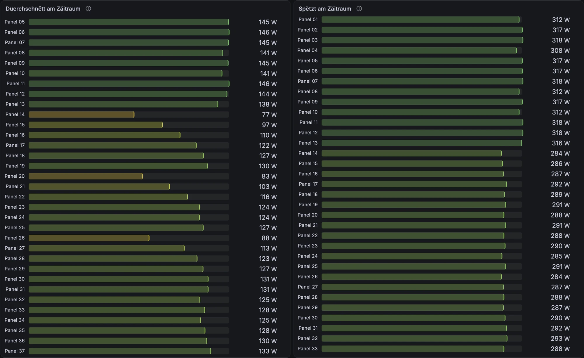
The heatmap over time and the per-panel averages are where it gets interesting. The peaks are almost identical across a roof, but the averages are not: panels 14, 15, 20, 21 and 26 on the garage roof average well below their neighbours. Same peak, lower average means partial shading during part of the day, not a defective module.

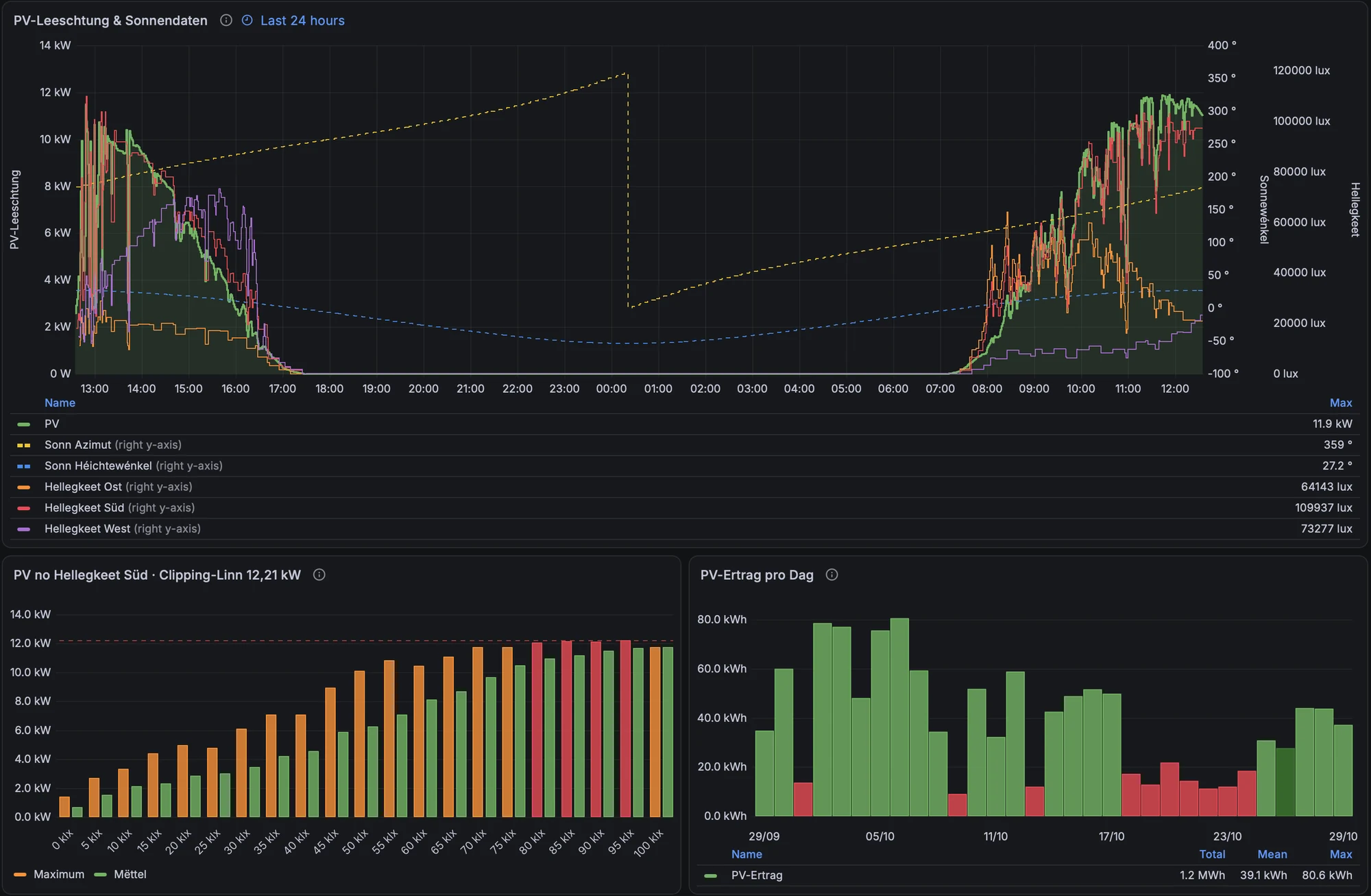
The array is deliberately over-panelled: 455 W modules on IQ8 microinverters that deliver at most about 330 W AC each, so 37 × 330 W ≈ 12.21 kW is the hard ceiling. Plotting PV power against the brightness measured on the south façade makes the clipping visible: above roughly 80 klx the maximum (orange) flattens at the clipping line. Over-panelling costs a little at noon in summer and gains a lot in the morning, the evening and in winter, which is what a self-consumption system needs.

3. Where does the PV go?

This was the hardest panel to get right, and the most instructive. The question is simple: of every kWh the roof produces, how much is used directly, how much goes into the Victron battery, how much into the Enphase battery, and how much is exported?

My first version used daily totals: direct use = PV − export − battery charging. It produced days with zero direct use on a 70 kWh day, which is physically impossible. The reason: daily totals cannot tell where energy came from. Two flows were counted twice:

• Evening battery export. When the Victron sells battery energy into the evening price peak, that energy appears in the export counter – but it had already been counted as PV going into the battery at midday.
• Battery-to-battery transfers. When the Enphase batteries discharge in the morning while the Victron is charging, the same kWh is counted as charging twice.

The fix is to do the bookkeeping minute by minute (in Flux, joining the Victron 1-minute data with the Enphase battery data): in each minute, export counts at most as much as the PV produced in that minute, battery charging counts at most what is left of PV after export, and the remainder is direct use. Battery export at night and transfers between batteries then drop out automatically. The four parts add up to the PV meter’s energy counter within about half a percent.

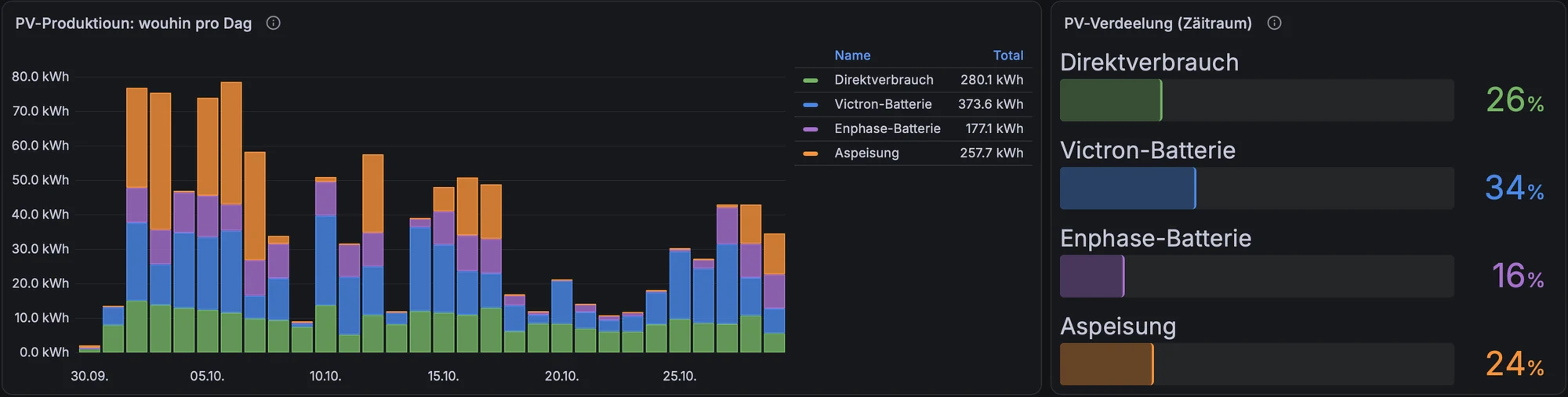
A side effect of building this panel: comparing the old and the new numbers quantifies how much energy is moved around rather than produced. Over three weeks, about 50 kWh of the export counter was battery energy sold in the evening, and several dozen kWh went into the Victron from the Enphase batteries or the grid. Every battery-to-battery kWh passes through two conversions and loses 10–15 %. That is an argument for configuring the two systems so they do not feed each other.

4. Grid: peaks and the 3 kW line

My grid tariff has a reference power of 3 kW; drawing more costs a surcharge. The peak panel shows the highest grid import per day, with a dashed line at 3 kW and red bars above it. The histogram counts minutes per 250 W bin, split into green (up to 3 kW) and red (above): 51 of roughly 41,500 minutes in 30 days. Export shows up to the left of zero.

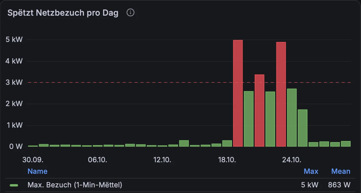
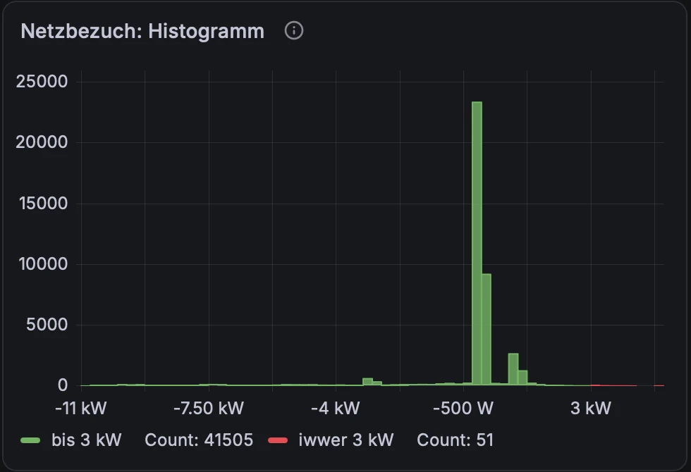
The grid operator assesses peaks as 15-minute averages, while these panels use 1-minute averages. A red bar is therefore a warning, not necessarily a surcharge: a three-minute spike may well average out below 3 kW over the quarter hour.

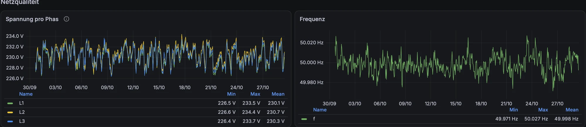
The Victron grid meter also measures voltage, frequency, neutral current and the voltage between neutral and protective earth. These are not needed for energy accounting, but they are cheap early-warning indicators: a slowly rising PEN voltage, for instance, can hint at a deteriorating neutral connection long before anything fails.

5. ESS control: what is the system doing, and why?

When the ESS is steered externally (grid setpoint, minimum SoC, peak shaving), it is easy to lose track of what is currently in effect. One row of tiles mirrors the relevant Ekrano settings, next to the spot price and the grid power. If the setpoint was left at an export value by a rule that crashed, it is visible at a glance.

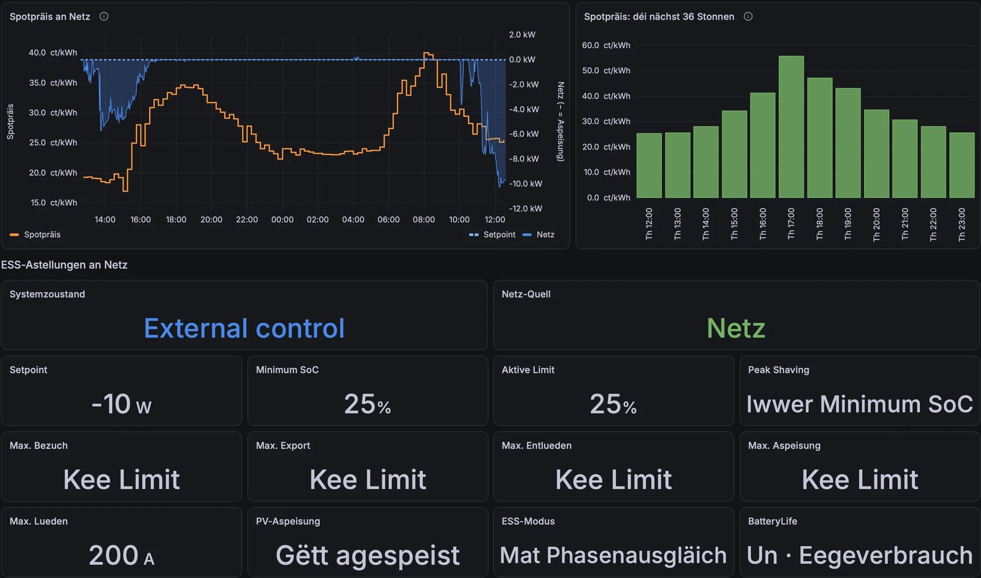
A state timeline shows the system state over the day (discharging, external control, etc.), the AC input source and the grid alarm. It is the fastest way to see whether an automation actually did what it was supposed to do at 18:00.

6. Batteries: throughput, cells, health

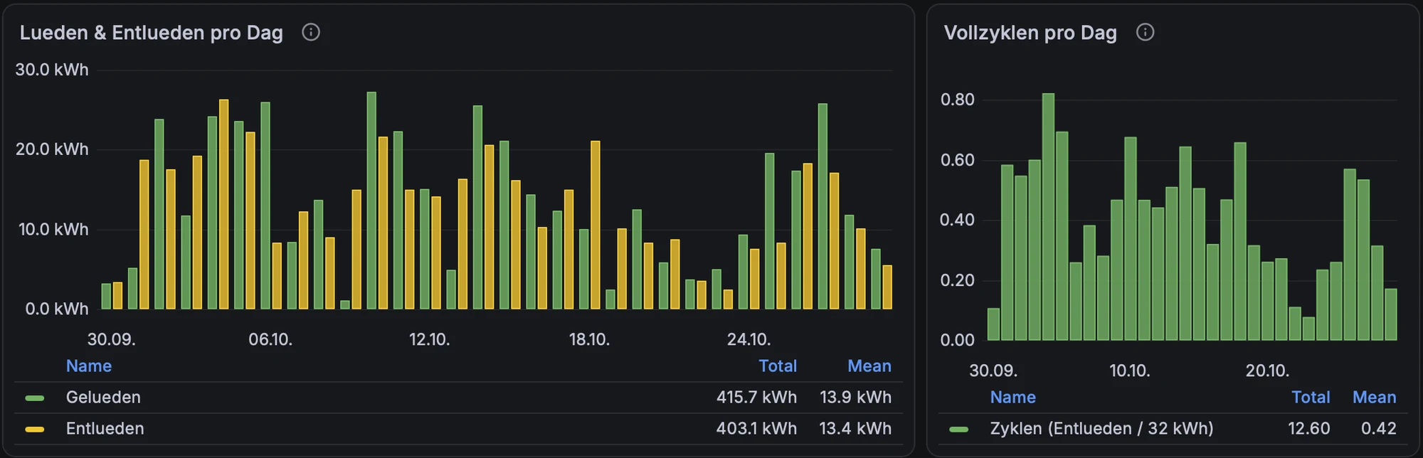
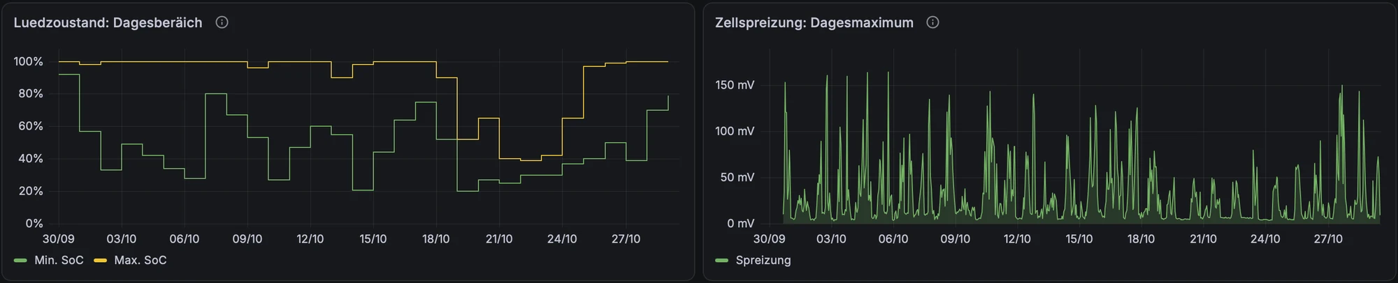
Daily charge and discharge energy and equivalent full cycles give a feel for how hard the battery is worked: here about 13–14 kWh per day and 12.6 full cycles in 30 days. The daily SoC range shows how deep the cycles go; in the darker second half of October, the Victron no longer reached 100 % every day.

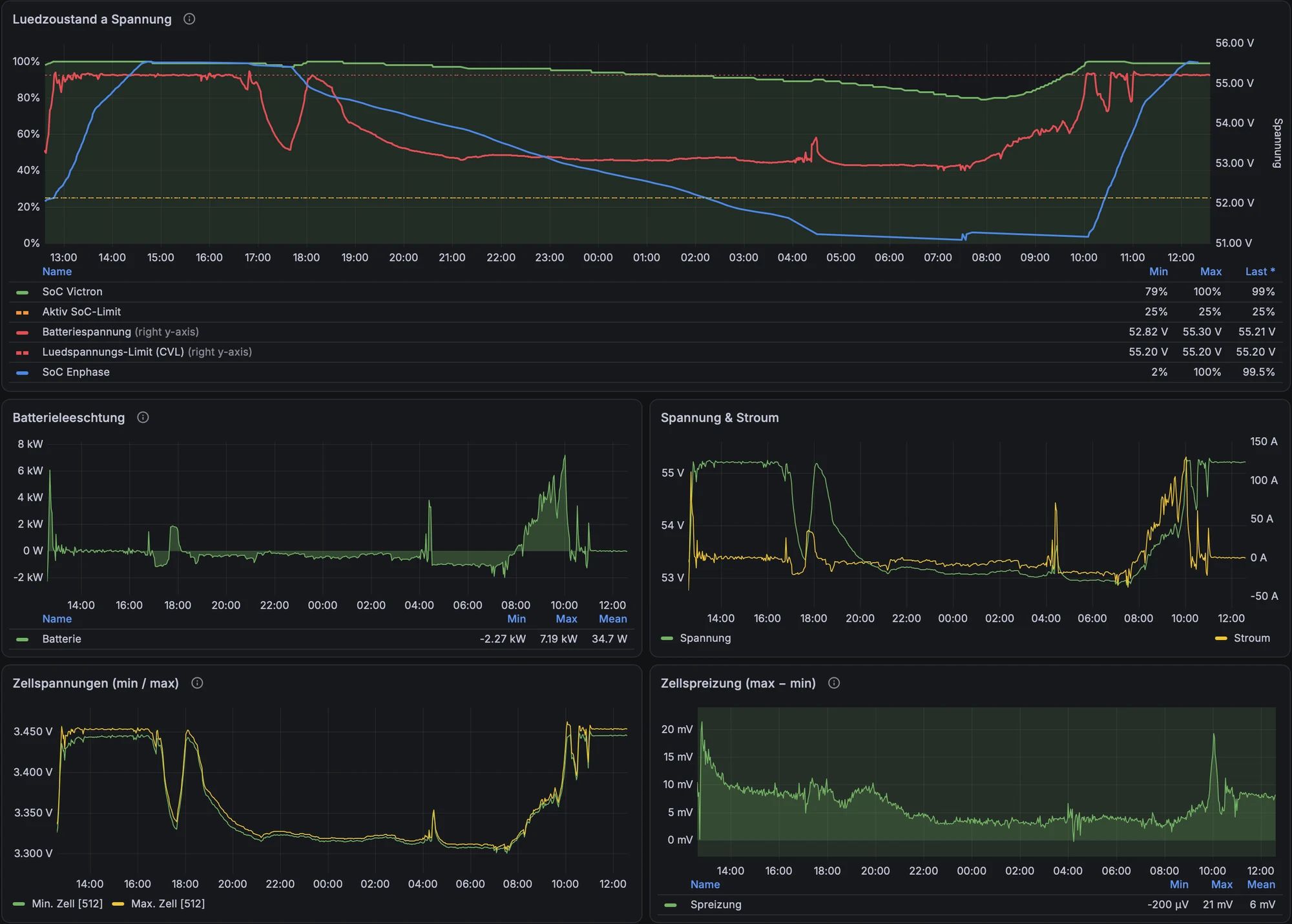
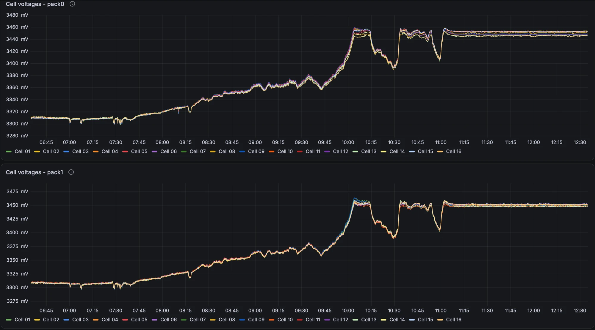
The 24-hour view combines SoC (Victron and Enphase), pack voltage and the charge voltage limit (CVL) on one chart, with power, current, minimum/maximum cell voltage and cell spread below. With LiFePO4, voltage is almost flat between roughly 20 and 90 % SoC and rises steeply only at the top, so the cell spread is mainly meaningful near full charge – which is exactly where it peaks.

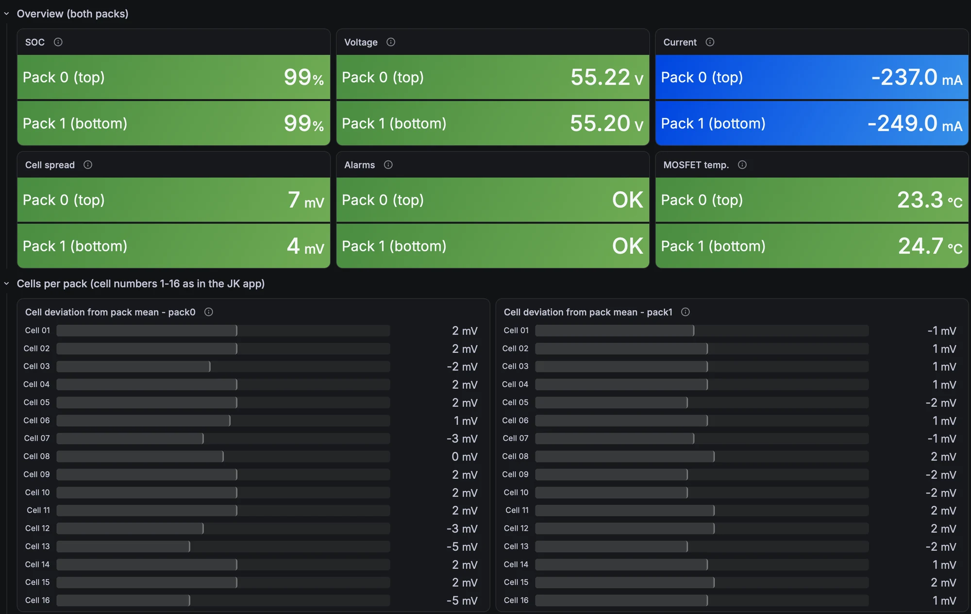
For the EEL packs, the JK BMS data go one level deeper. The overview shows SoC, voltage, current, cell spread, alarms and MOSFET temperature per pack; the bars below show each cell’s deviation from the pack mean. ±5 mV at rest is a healthy, well-balanced pack.

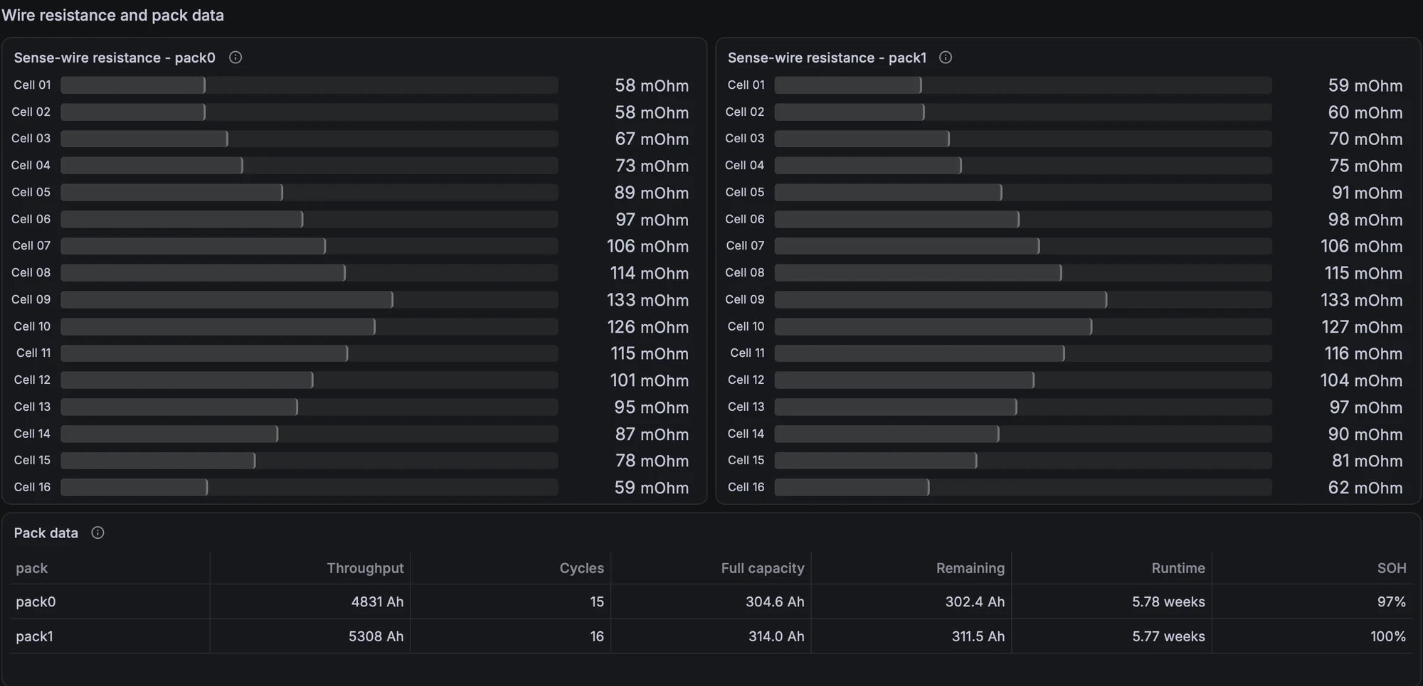
Two panels I would recommend to anyone with a JK BMS. First, the sense-wire resistance per cell: it is the same, symmetrical pattern in both packs (highest around cell 9), so it reflects wire length rather than a bad connection – but a single cell suddenly deviating from that pattern would point to a loosening terminal. Second, the pack data table with throughput, cycles, full capacity and state of health.

7. Where does the base load go?

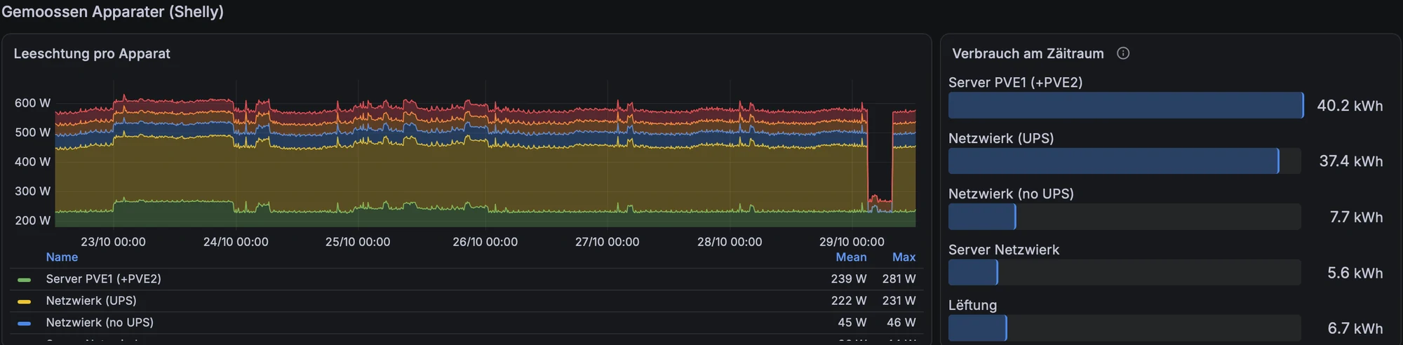
Finally, individual consumers measured with Shelly plugs. In my case the servers and the network equipment run at around 500 W around the clock, roughly 12–13 kWh a day. That is the single biggest lever on the night-time battery drain, and it is also why consumption figures that miss the server circuit are badly off.

Lessons learned

• Do not trust daily totals for energy flows. As soon as batteries export or charge each other, only a per-minute calculation tells you where the PV went.
• Never sum percentages. A legend that showed 2013 % “total” self-sufficiency taught me that one. And an unweighted mean of daily ratios lies too: weight by kWh.
• Self-consumption in percent rewards a smaller PV array. In kWh, it is the number that matters economically. Autarky in percent is the meaningful ratio.
• Meters have noise. The PV meter showed 6.5 W at night: CT offset and the microinverters’ filter capacitors, not moonlight. A small dead band (below 15 W shows as 0) keeps the live view honest without touching the stored data.
• Do not draw lines across gaps for regularly sampled data; show the gap. Values from systems that only report on change (openHAB) are step lines that hold their last value.
• Two y-axes with the same unit mislead. If both are °C or both are W, use one axis.
• Know your CTs. Before interpreting consumption or autarky, verify what each clamp actually measures. Mine still need work, and the post shows only what is coherent today.

Stack: Victron Venus OS on Ekrano GX → MQTT → Telegraf → InfluxDB 2; Enphase Envoy and JK BMS → openHAB / MQTT → InfluxDB 2; Grafana 13. All self-hosted.