After the electricity side (Monitoring a Victron + Enphase hybrid system with Grafana), this is the other half of the house: a gas condensing boiler with solar thermal support for hot water, room-by-room heating control over KNX, and the water supply with its softener. The goal is the same as before: not pretty pictures, but panels that answer concrete questions. How much gas does the house need per degree of cold? Which room is the bottleneck? Is the boiler cycling too often? And would a heat pump pay off?

Dashboard labels are in Luxembourgish; I translate the important ones.

The setup

• Boiler: gas condensing boiler with an RC35 controller, read out via EMS-ESP over MQTT (flow and return temperatures, burner power, starts, run time, pressure, hot water).
• Solar thermal: collector, two storage temperatures (bottom and top) and the solar pump, also via EMS-ESP.
• Rooms: KNX room controllers and heating actuators deliver room temperatures and the valve demand per room.
• Meters: gas and electricity from the smart meter’s P1 port, water from the water meter, plus the softener’s own data.
• Weather: a local weather station (temperature, humidity, pressure, rain, brightness on three façades).
• Path: everything goes into openHAB, is persisted to InfluxDB 2 and visualised in Grafana 13. Self-hosted, no vendor cloud needed.

1. The building: gas per degree of cold

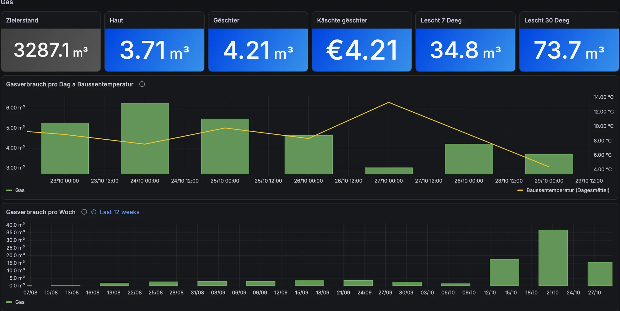
If I had to keep only one heating panel, it would be this one. Each dot is one day: gas consumption against the daily mean outdoor temperature, over a year, with a linear regression. The relationship is remarkably clean, and it tells you a lot about the building:

• The line reaches zero at about 16 °C: that is the heating limit temperature. Above it, the house heats itself from internal and solar gains.
• The slope is about 0.71 m³ per day and kelvin. With 10.8 kWh/m³ and a boiler efficiency of 0.92, that is roughly 7 kWh of heat per kelvin per day, or about 0.3 kW per kelvin.
• At a design temperature of around −10 °C (26 K below the heating limit), that gives a heat load of roughly 8 kW. This is the number that matters for sizing a heat pump, and it is measured, not taken from a standard calculation.

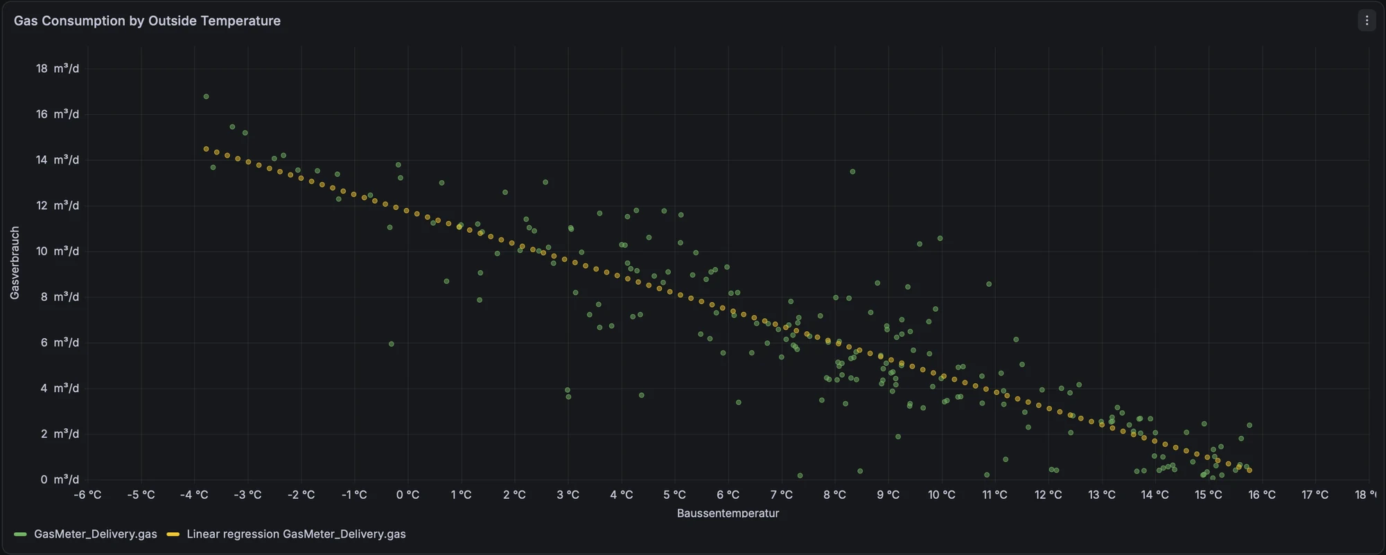
This is an estimate: the regression mixes in hot water (partly covered by solar), and days with unusual use (guests, holidays) scatter. For sizing decisions I would still round up, not down.

2. Rooms: where does the heat go?

The heating actuators report a valve demand per room. Shown as a state timeline per day (grey below 5 %, then blue, yellow, orange, red from 75 %), it shows at a glance which rooms actually need heat. The averages and the valve hours over the period underneath turn that into numbers.

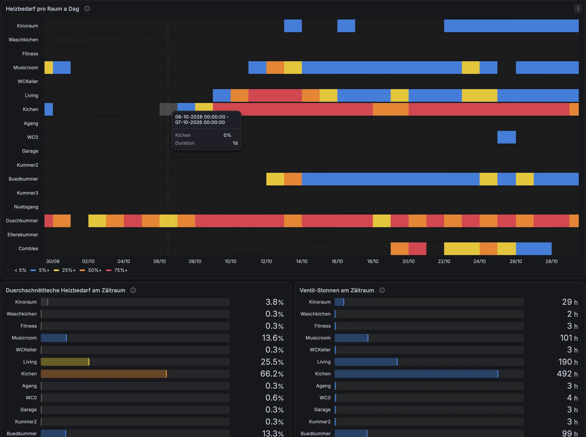
The surprise here was the kitchen: its valve is open most of the time (66 % on average, almost 500 valve hours in 30 days), while the living room next to it needs 25 %. A room whose valve is permanently open is either set warmer than the others, under-supplied hydraulically, or losing heat somewhere. It is the first candidate for hydraulic balancing, and the first room to look at if the flow temperature is ever lowered for a heat pump: the room with the highest demand determines the flow temperature the whole house needs.

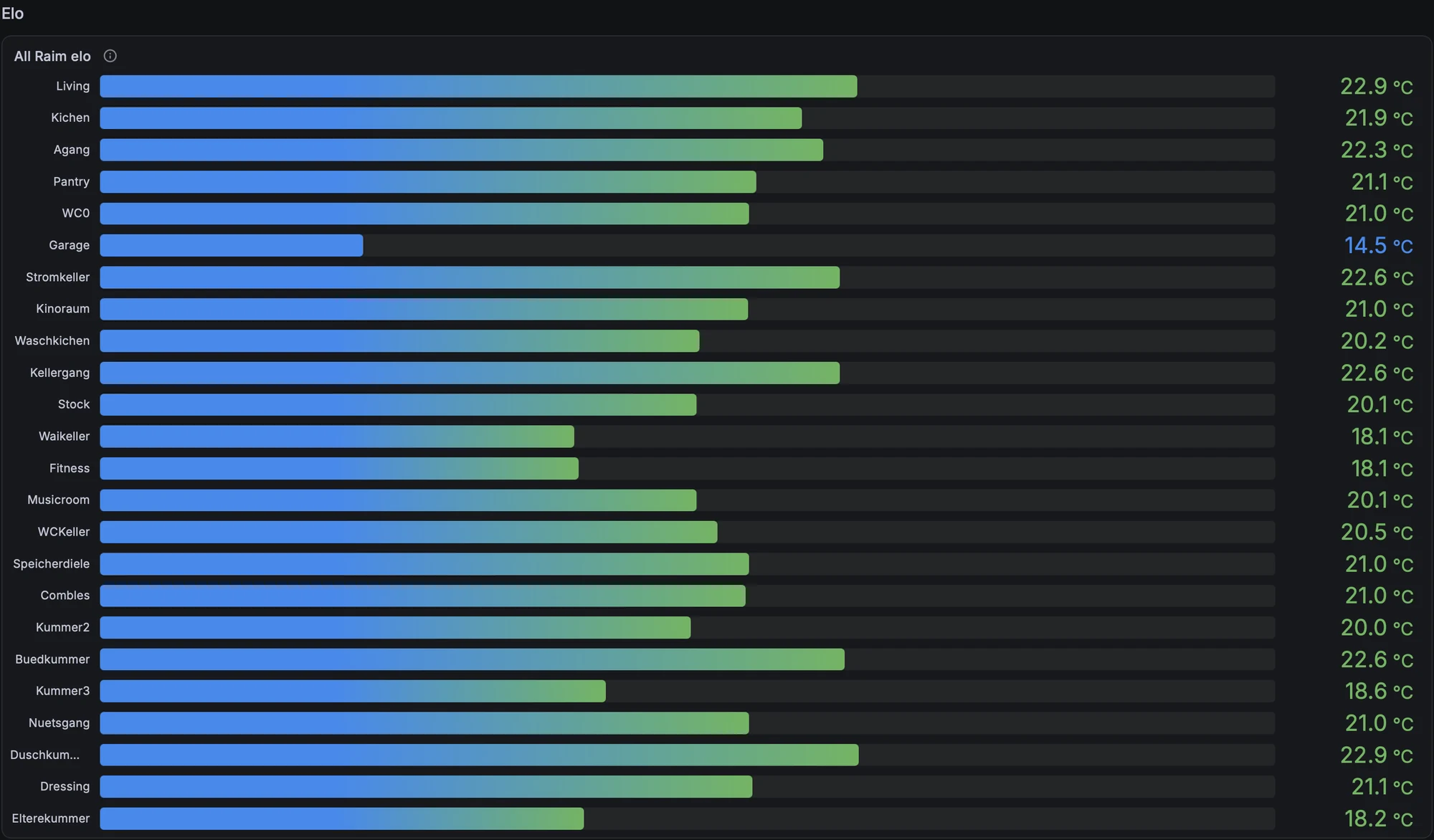
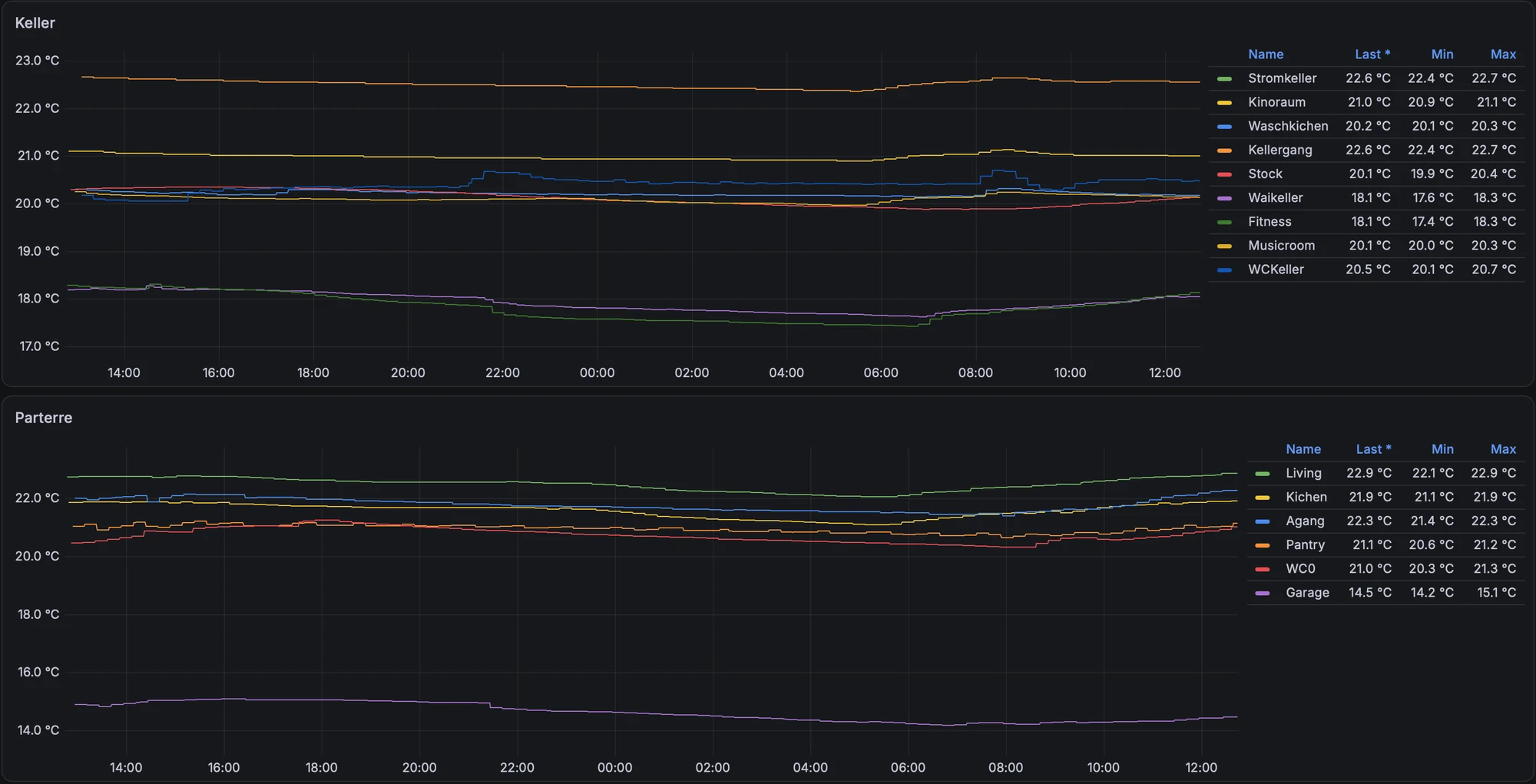
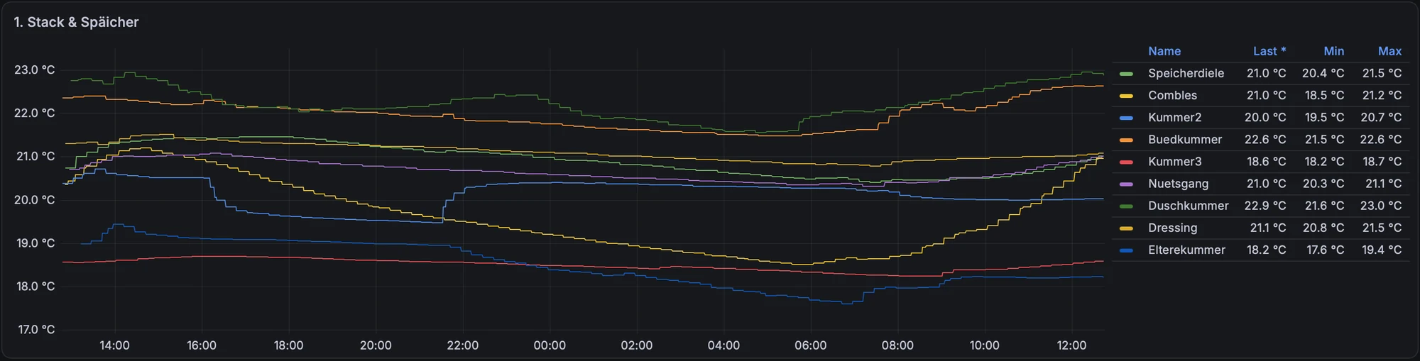
Room temperatures complete the picture: a bar per room for the current state, and one chart per floor over 24 hours. Unheated or lightly heated rooms (garage, utility cellar, bedrooms kept cooler) are immediately visible.

3. Boiler: flow temperatures and cycling

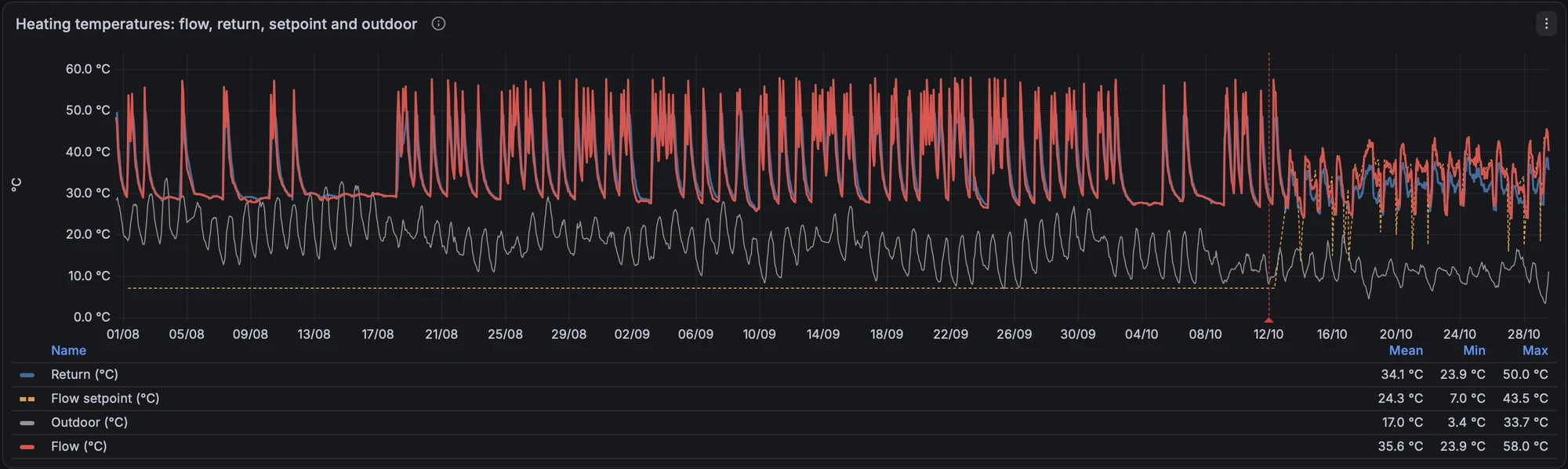
Flow, return, flow setpoint and outdoor temperature on a single °C axis (an earlier version had two axes, which made the gap between outdoor and flow temperature look smaller than it is). In summer the heating circuit is switched off manually and only hot water is produced; the flow setpoint then drops to its minimum. From mid-October the heating curve takes over: roughly 46 °C minus 0.84 × outdoor temperature, with a floor at 33 °C.

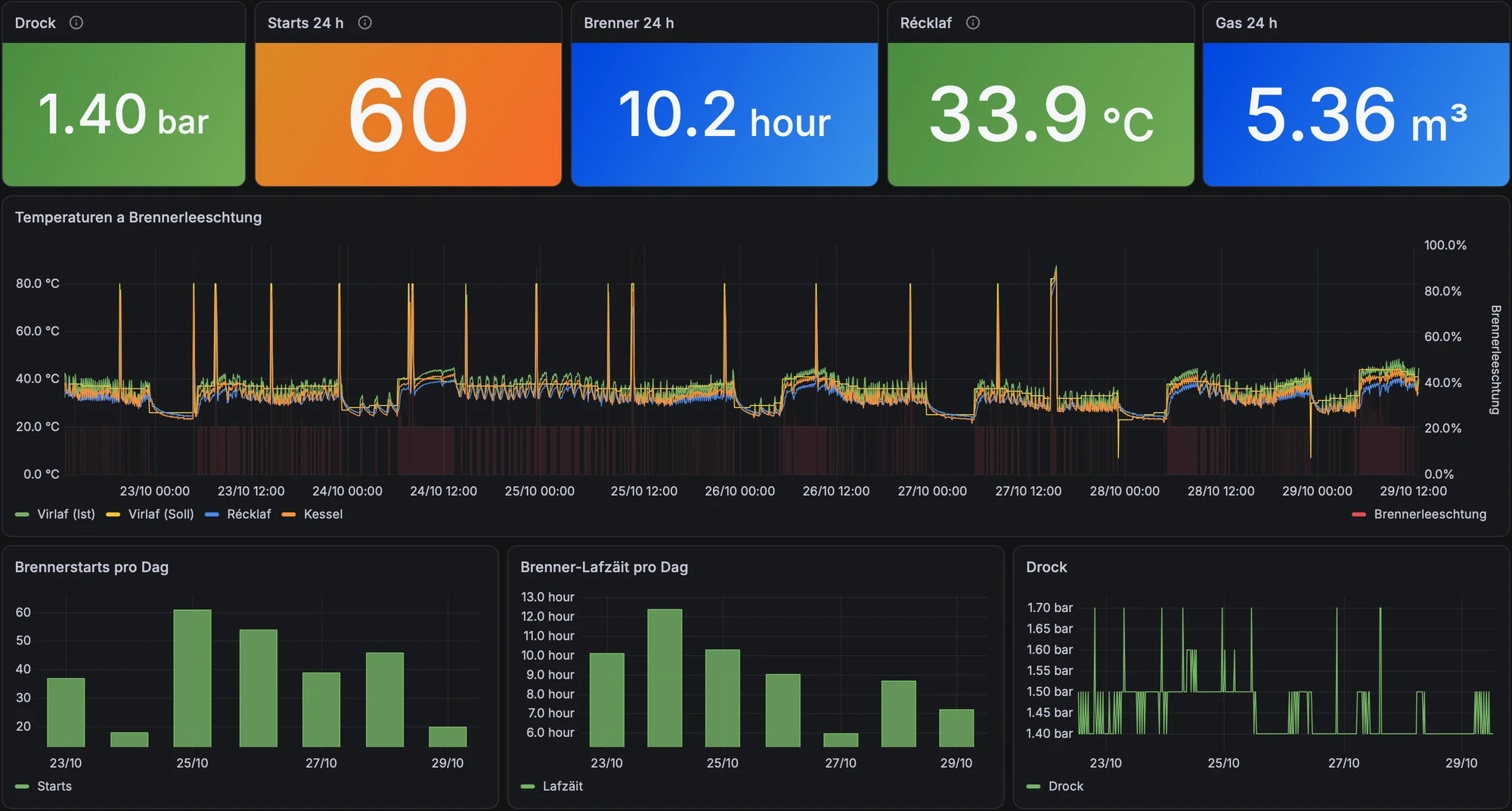
The boiler view adds pressure, burner starts, burner hours, return temperature and gas per day. Two things are worth watching here:

• Return temperature: around 34 °C, well below the roughly 55 °C dew point of the flue gas. The boiler is condensing, as it should.
• Burner starts: up to 60 starts a day with about 10 hours of burner time means many short cycles. Short cycling costs efficiency and wears the burner. It is a sign that the boiler’s minimum output is larger than the house needs on mild days; burner hysteresis and the minimum modulation are worth a look.

4. Hot water and solar thermal

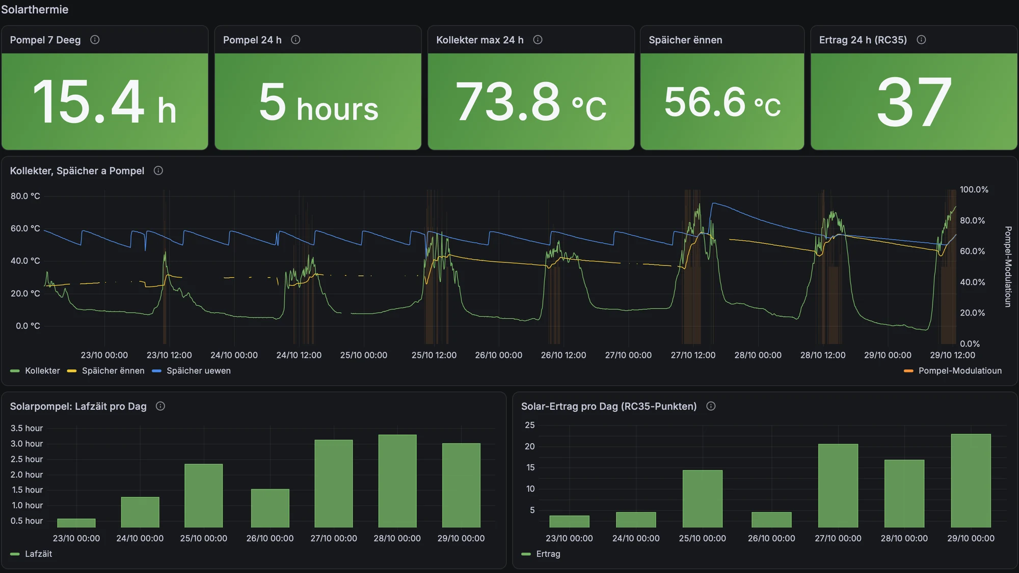
The solar section shows the collector against the bottom and top of the storage tank, and the pump modulation. On sunny days in late October the collector still reached 70 °C and the solar pump ran three hours a day. The yield is shown in the controller’s own units (“RC35 points”), which are not kWh; it is useful for comparing days, not for an energy balance.

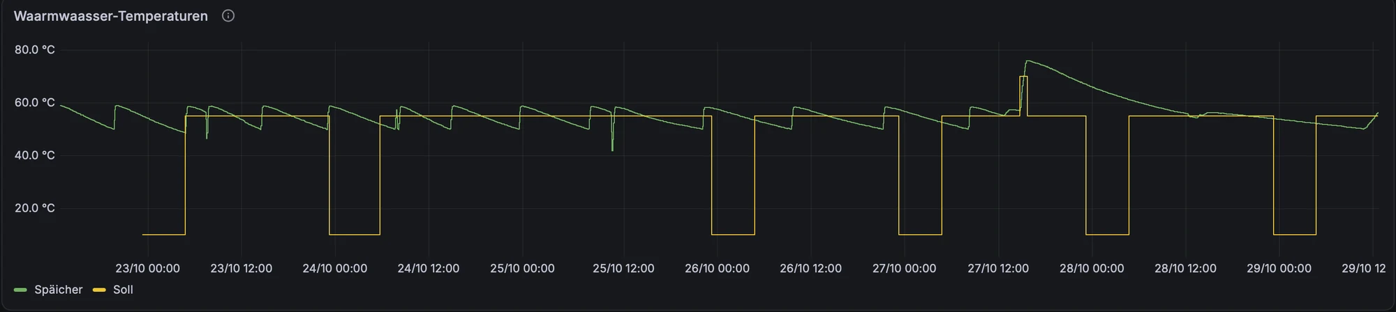
The hot-water chart shows the storage temperature against its setpoint. The setpoint drops at night (night setback), so the boiler does not reheat the tank for nobody; the tank cools slowly and is reheated in the morning, or by the sun.

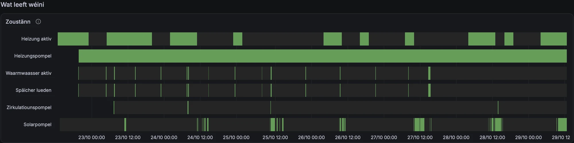
Finally, a state timeline of what is running when: heating active, heating pump, hot water active, storage charging, circulation pump and solar pump. It is the quickest way to check that automations and time programs actually do what they are meant to do.

5. Would a heat pump pay off?

With measured daily gas consumption and outdoor temperatures, the heat-pump question becomes a calculation instead of a sales pitch. The energy dashboard converts gas to delivered heat (m³ × 10.8 kWh/m³ × 0.92), models a daily COP from the outdoor temperature and the house’s actual heating curve, and compares running costs with prices I can change as variables. The full model and every price component are documented in a text panel next to the result.

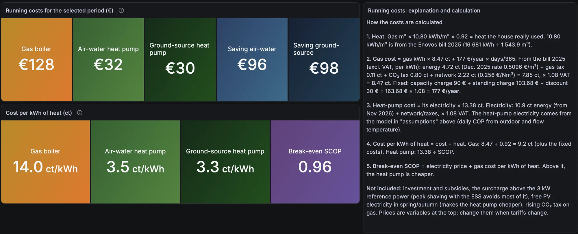
Read these numbers with the period in mind. This screenshot covers 90 days that are mostly summer. With little gas used, the fixed gas costs (177 € per year, pro rata) dominate, which pushes the gas price per kWh of heat to 14 ct and the break-even SCOP below 1. Over a full heating season the comparison is less extreme: without fixed costs, a kWh of heat from gas costs about 9.2 ct, and the heat pump wins from a SCOP of about 1.45. Either way the margin is large, but the honest figure comes from a whole year, not from a quarter.

6. Indoor climate and weather

The weather station supplies outdoor temperature, humidity, pressure, rain and brightness on three façades. The same brightness data also drive the PV analysis on the electricity side.

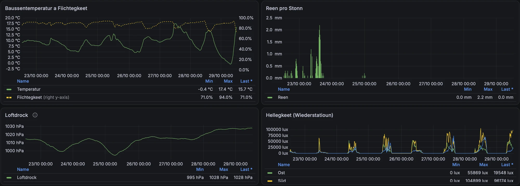
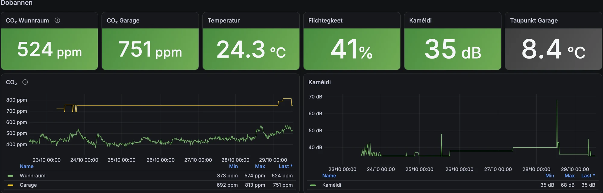
Indoors, CO₂ in the living area is the best single indicator of whether the ventilation keeps up; here it stays between roughly 370 and 570 ppm. The dew point in the garage helps judge condensation risk in an unheated space.

7. Water and softener

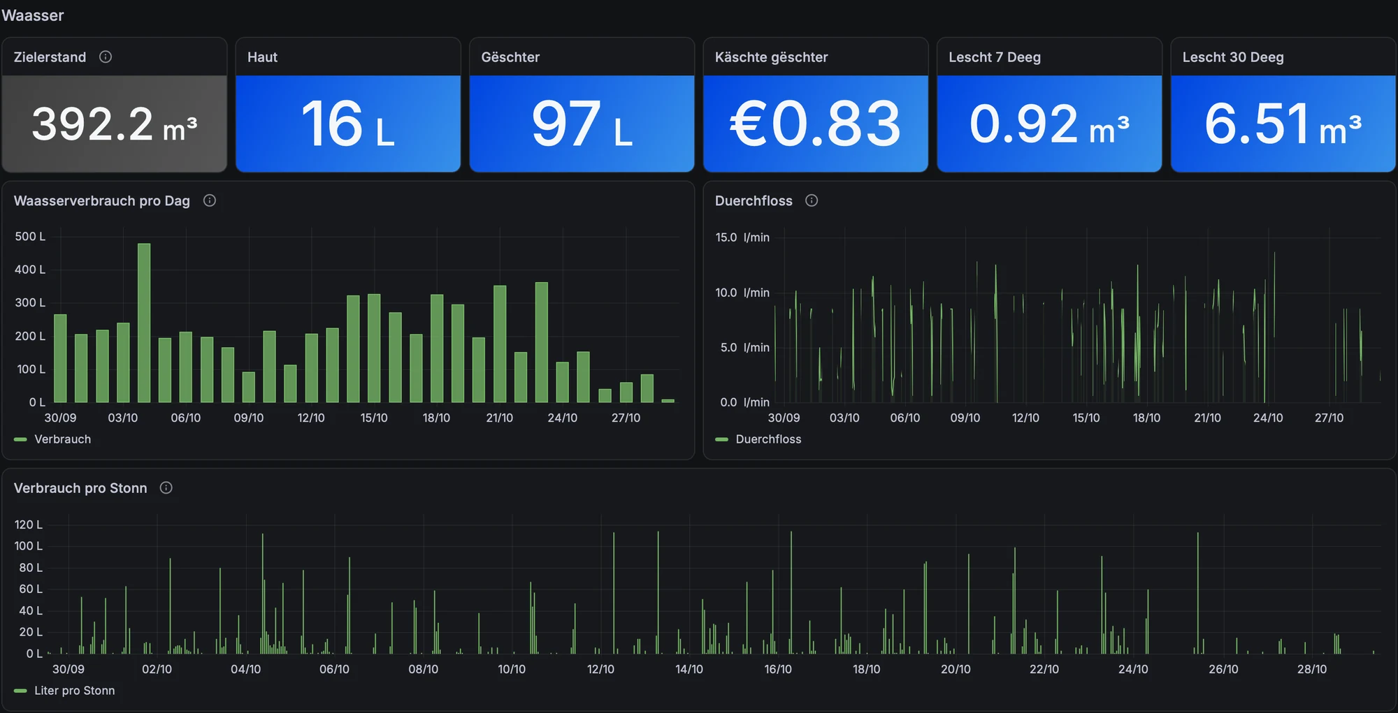
Water is not heating, but it shares the dashboards’ folder and the same questions: how much, when, and is anything leaking? Daily consumption, flow and consumption per hour make an unnoticed leak visible quickly: a leak shows up as consumption during hours when nobody uses water.

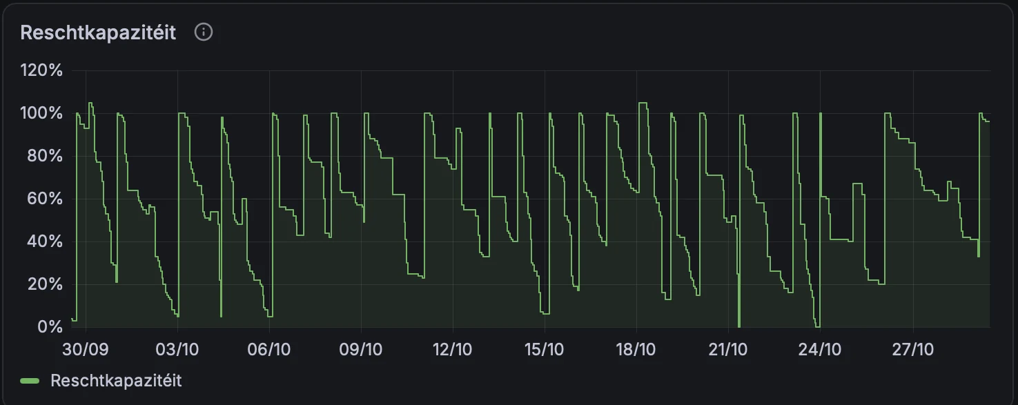
The softener reports its remaining capacity, the next regeneration, regenerations over 30 days, total salt and the next maintenance. The remaining-capacity sawtooth shows the regeneration rhythm: 20 regenerations in 30 days, at roughly 200 L of water a day.

Lessons learned

• Gas per degree is the most valuable heating chart. It gives the heating limit temperature and the building’s heat loss coefficient, and with them a measured heat load for heat-pump sizing.
• Valve demand per room beats room temperature for diagnosis. A room at the right temperature with a permanently open valve is the real bottleneck, and it sets the flow temperature for the whole house.
• Count burner starts. Run time alone hides short cycling.
• Use one axis for one unit. Flow and outdoor temperature belong on the same °C scale; otherwise the chart lies about the distance between them.
• Mind the period in cost comparisons. Fixed costs make a summer quarter look very different from a winter.
• Controller units are not kWh. Solar “points” from the controller are fine for comparing days, not for an energy balance.

Stack: EMS-ESP (boiler, solar), KNX (rooms), P1 smart meter (gas, electricity), weather station, water meter and softener → openHAB → InfluxDB 2 → Grafana 13. All self-hosted.